Numpy
“Numpy” is a important module in Python for doing numerical computations in a optimized way. Numpy stands for “numerical python”. Numpy is used for working with arrays as a Python library, which has functions for working in domain of linear algebra, fourier transform, and matrices. It also contains all the usual math functions, its own version of random module, and its own special data types, like “arrays”.
In numpy, an “array” is a lot like a list except arrays MUST hold ectries of the SAME data type, which works exactly like an array insome other language like C, C++, and Java. Nmoy takes advantage of its homogeneity to store and process arrays faster than lists. In addition, we can do element-wise operations with arrays easily. The array object in NumPy is called ndarray, it provides a lot of supporting functions that make working with ndarray very easy. NumPy arrays are stored at one continuous place in memory unlike lists, which means processes can access and manipulate them very efficiently.
# numpy module is not preinstalled in Python so we need to import it
import numpy as np
# if an error is raised: ModuleNotFoundError: No module named 'numpy'
# try to run "pip install numpy" in command line

# a 1-dimensional array, or "vector"
# <-3, 5, 4>
>>> A1 = np.array([-3, 5, 4])
>>> print(A1)
[-3  5  4]
# notice that when we define a numpy array, we need to put a list inside

# a 2-dimensional array, or "matrix"
# [4, 1]
# [3, 9]
>>> A2 = np.array([[4, 1], [3, 9]])
>>> print(A2)
[[4 1]
 [3 9]]
# notice that when defining a 2-d array, it needs to be lists in list

# vectorization: numpy allows to operate on all elements of an array at once
>>> print(3*A1)   # multiply the elements in the array by 3
[-9 15 12]
>>> print(A1**2)    # square all the elements
[ 9 25 16]
>>> print(np.sin(A1))     # take the sin values of all the elements
[-0.14112001 -0.95892427 -0.7568025 ]
>>> A3 = np.array([-0.43, 1, 0.9])
>>> print(A1 + A3)        # add the coresponding entries
[-3.43  6.    4.9 ]
>>> print(A1 * A3)        # multiple the coresponding entries
[1.29 5.   3.6 ]

# Numpy has several methods for wasily generating large arrays
# arange(start,end,step,dtype=)
# generate a array from start to end (not include) in step where data type is dtype
>>> A4 = np.arange(3, 20, 2)
>>> print(A4)
[ 3  5  7  9 11 13 15 17 19]

# linspace(start,end,num)
# generate num evenly spaced samples, calculated over the interval [start,end)
>>> A5 = np.linspace(0, 10, 100)
>>> print(A5)
[ 0.          0.1010101   0.2020202   0.3030303   0.4040404   0.50505051
  0.60606061  0.70707071  0.80808081  0.90909091  1.01010101  1.11111111
  1.21212121  1.31313131  1.41414141  1.51515152  1.61616162  1.71717172
  1.81818182  1.91919192  2.02020202  2.12121212  2.22222222  2.32323232
  2.42424242  2.52525253  2.62626263  2.72727273  2.82828283  2.92929293
  3.03030303  3.13131313  3.23232323  3.33333333  3.43434343  3.53535354
  3.63636364  3.73737374  3.83838384  3.93939394  4.04040404  4.14141414
  4.24242424  4.34343434  4.44444444  4.54545455  4.64646465  4.74747475
  4.84848485  4.94949495  5.05050505  5.15151515  5.25252525  5.35353535
  5.45454545  5.55555556  5.65656566  5.75757576  5.85858586  5.95959596
  6.06060606  6.16161616  6.26262626  6.36363636  6.46464646  6.56565657
  6.66666667  6.76767677  6.86868687  6.96969697  7.07070707  7.17171717
  7.27272727  7.37373737  7.47474747  7.57575758  7.67676768  7.77777778
  7.87878788  7.97979798  8.08080808  8.18181818  8.28282828  8.38383838
  8.48484848  8.58585859  8.68686869  8.78787879  8.88888889  8.98989899
  9.09090909  9.19191919  9.29292929  9.39393939  9.49494949  9.5959596
  9.6969697   9.7979798   9.8989899  10.        ]

# we can also generate random arrays using the random module inside the munpy module
# random.random(n)
# generate a array with n random floats between [0,1)
>>> A6 = np.random.random(20)
>>> print(A6)
[0.23570986 0.80712129 0.85676756 0.66425472 0.22152999 0.61819233
 0.55393604 0.16557989 0.34441581 0.16123907 0.119222   0.21565709
 0.96264147 0.19140327 0.50218279 0.66988965 0.67286977 0.6767917
 0.86861928 0.43622269]

# random.random([row, col])
# generate a matrix with random float between [0,1) where the matrix is in row rows and col columns
>>> A7 = np.random.random([3,3])
>>> print(A7)
[[0.43290007 0.17095905 0.94986462]
 [0.76059458 0.04115602 0.60096588]
 [0.78158437 0.44977247 0.70040134]]

# random.randint(low,high,size)
# generate a size array of random integers between [low,high)
# if high is not given, the number will be generated between[0,low)
>>> A8 = np.random.randint(8, size=10)
>>> print(A8)
[2 4 0 0 1 6 4 2 7 2]
Matplotlib
Matplotlin in Python stands for mathematical plotting library. It is a low level graph plottign library that serves as a visualization urility. Matplotlib is very useful for making graphs and having a lot of control over how the graphs look. There are many submodules under matplotlib. The most common used is pyplot submodule. The matplotlib is not preinstalled in Python, we can use “pip install matplotlib” in command line, and import it into our python program.
# plot some discrete points
>>> import matplotlib.pyplot as plt
>>> X = [3, 5, -2]
>>> Y = [1, 0.8, -4]
>>> plt.plot(X, Y, "ro")
[<matplotlib.lines.Line2D object at 0x000001F0823E65C0>]
>>> plt.show()
# we can use plt.savefig("name_of_fig") to save it in png format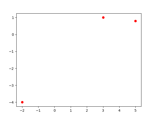
Notice that in the plot() method, there is a string that controls the style of the image that we created. There are actually more options for colors and styles.
# colors: r, g, b, c, m, y, w, k
# linestyles: o, -, --, :, -.
# we can combine the color with linestyle to create different images
# we can also use numpy module to create X and Y values

# making random points and plotting them
>>> import matplotlib.pyplot as plt
>>> import numpy as np
>>> x_rand = np.random.random(100)
>>> y_rand = np.random.random(100)
>>> plt.plot(x_rand, y_rand, "go")
[<matplotlib.lines.Line2D object at 0x000001F0838A5B40>]
>>> plt.show()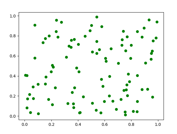
# make the letter E with a plot
>>> import matplotlib.pyplot as plt
>>> import numpy as np
>>> X = [3, 0, 0, 3, 0, 0, 3]
>>> Y = [6, 6, 3, 3, 3, 0, 0]
>>> plt.plot(X, Y, "r-")
[<matplotlib.lines.Line2D object at 0x000001F086113430>]
>>> plt.show()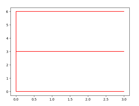
# we can also plot some functions
>>> import matplotlib.pyplot as plt
>>> import numpy as np
>>> x = np.arange(-np.pi, np.pi, 0.01)
>>> y = np.cos(x)
>>> plt.plot(x, y, "r")
[<matplotlib.lines.Line2D object at 0x000001F086A1B0A0>]
>>> plt.show()

# we can even plot multiple functions in a single graph
>>> x = np.arange(-np.pi, np.pi, 0.01)
>>> y1 = np.sin(x)
>>> y2 = x**2 - 5
>>> y3 = np.exp(x)
>>> plt.plot(x, y1, 'r', x, y2, 'g', x, y3, 'b')
[<matplotlib.lines.Line2D object at 0x000001F086AA7430>, <matplotlib.lines.Line2D object at 0x000001F086AA7400>, <matplotlib.lines.Line2D object at 0x000001F086AA7460>]
>>> plt.show()

# colors and markers can be specified in other ways
# for instance, we use (r, g, b) tuple to specify the amount of red, green, and blue

# specify colors in different way
>>> import matplotlib.pyplot as plt
>>> import numpy as np
>>> x = np.random.random(100)
>>> y = np.random.random(100)
>>> for i in range(100):
...     plt.plot(x[i], y[i], marker='o', color=((x[i]+y[i])/2, 0, 1-(x[i]+y[i])/2))
...
>>> plt.show()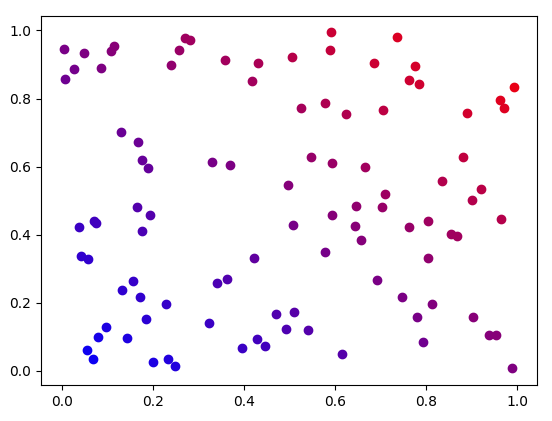
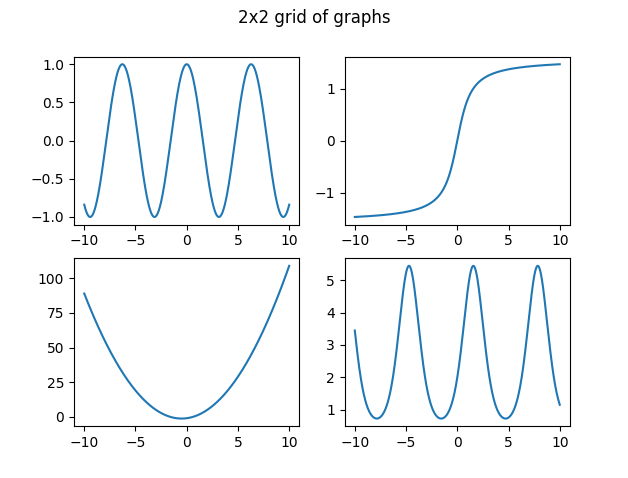
# instead of plotting all the function in a single graph, we can make them in a grid

# graphing on a 2x2 grid
>>> import matplotlib.pyplot as plt
>>> import numpy as np
>>> fig, ax = plt.subplots(2, 2)
>>> x = np.linspace(-10, 10, 1000)
>>> y1 = np.cos(x)
>>> y2 = x**2+x-1
>>> y3 = np.arctan(x)
>>> y4 = 2*np.exp(np.sin(x))
>>> ax[0][0].plot(x, y1)
[<matplotlib.lines.Line2D object at 0x000001F08777C610>]
>>> ax[1][0].plot(x, y2)
[<matplotlib.lines.Line2D object at 0x000001F08777C670>]
>>> ax[0][1].plot(x, y3)
[<matplotlib.lines.Line2D object at 0x000001F08777C940>]
>>> ax[1][1].plot(x, y4)
[<matplotlib.lines.Line2D object at 0x000001F08777CBE0>]
>>> fig.suptitle("2x2 grid of graphs")
Text(0.5, 0.98, '2x2 grid of graphs')
>>> plt.show()
# there are some other graphs that we can make through pyplot
>>> import matplotlib.pyplot as plt
>>> import numpy as np
# bar chart
>>> labels = np.array(["apple", "vegatable", "candy", "soda"])
>>> bar_sizes = np.array([10, 15, 8, 13])
>>> plt.bar(labels, bar_sizes)
<BarContainer object of 4 artists>
>>> plt.show()
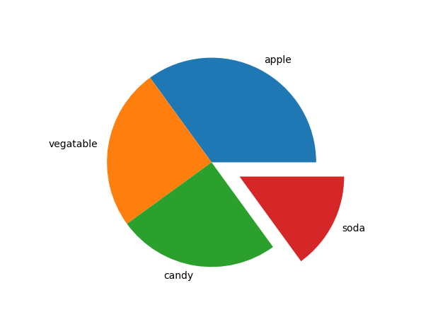
# pie chart
>>> sizes = np.array([35, 25, 25, 15]) # they need to add up to 100
>>> my_labels = ["apple", "vegatable", "candy", "soda"]
>>> my_explode = [0, 0, 0, 0.3] # select a category to be explode
>>> plt.pie(sizes, labels=my_labels, explode=my_explode)
([<matplotlib.patches.Wedge object at 0x000001F087CBAB00>, <matplotlib.patches.Wedge object at 0x000001F087CBAA40>, <matplotlib.patches.Wedge object at 0x000001F087CBB3D0>, <matplotlib.patches.Wedge object at 0x000001F087CBB850>], [Text(0.4993895680663529, 0.9801071672559597, 'apple'), Text(-1.086457168210212, 0.17207795223283895, 'vegatable'), Text(-0.172077952232839, -1.086457168210212, 'candy'), Text(1.2474091219621306, -0.6355867229935397, 'soda')])
>>> plt.show()
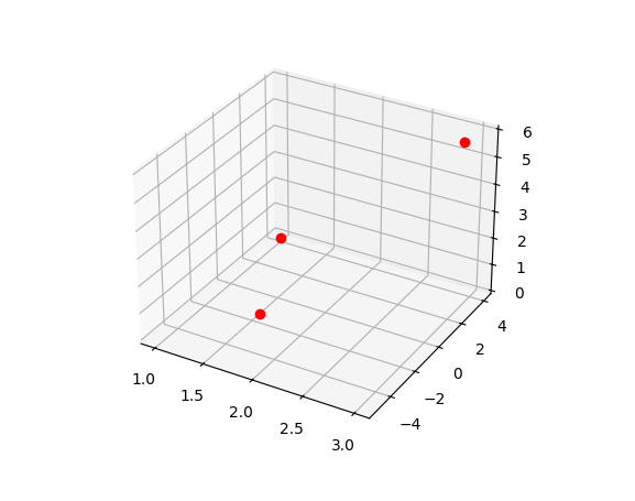
# points in 3D
>>> x = [1, 2, 3]
>>> y = [4, -5, 3]
>>> z = [0, 2, 6]
>>> ax = plt.axes(projection='3d')
>>> ax.plot3D(x, y, z, "ro")
[<mpl_toolkits.mplot3d.art3d.Line3D object at 0x000001F087D23670>]
>>> plt.show()
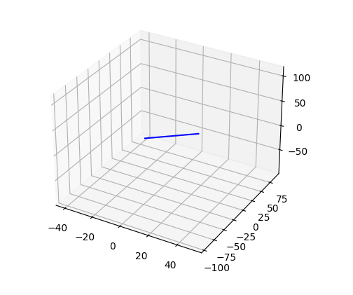
# line in 3D (parametrized curve)
>>> t = np.linspace(-15, 15, 2001)
>>> x = 3*t + 5
>>> y = -6*t - 3
>>> z = 7*t + 9
>>> ax = plt.axes(projection='3d')
>>> ax.plot3D(x, y, z, 'b-')
[<mpl_toolkits.mplot3d.art3d.Line3D object at 0x000001F087C14310>]
>>> plt.show()
# sueface in 3D
# a surface of z = 1/2*x*y^2 + sin(x*y)
# we need to use meshgrid() to turn our line of x, y values into a grid of x, y values
>>> x = np.linspace(-10, 10, 101)
>>> y = np.linspace(-10, 10, 101)
>>> X, Y = np.meshgrid(x, y)
>>> Z = 1/2*X*Y**2 + np.sin(X*Y)
>>> ax = plt.axes(projection='3d')
>>> ax.plot_wireframe(X, Y, Z, color='red')
<mpl_toolkits.mplot3d.art3d.Line3DCollection object at 0x000001F087623FA0>
>>> plt.show()